"It will without doubt have come to your Lordship's knowledge that a considerable change of climate, inexplicable at present to us, must have taken place in the Circumpolar Regions, by which the severity of the cold that has for centuries past enclosed the seas in the high northern latitudes in an impenetrable barrier of ice has been during the last two years, greatly abated.(This) affords ample proof that new sources of warmth have been opened and give us leave to hope that the Arctic Seas may at this time be more accessible than they have been for centuries past, and that discoveries may now be made in them not only interesting to the advancement of science but also to the future intercourse of mankind and the commerce of distant nations."
President of the Royal Society, London, to the Admiralty, 20th November, 1817 [13]
Introduction
The `Arctic' is a general term applied to all the lands, ocean, and ice north of the Arctic Circle at 67°N. It includes the northern Canadian Archipelago, most of Greenland, the Norwegian Sea, the Arctic Ocean, and the northern coastlines of Russia, Scandinavia, Canada and Alaska.
As the above extract from 1817 shows, the
ebb and flow of Arctic ice extent and mass is nothing new, as can be
expected from such a dynamic and changing ocean/ice environment.
This is also the region which climate models indicate will receive a much larger warming from an enhanced greenhouse effect than would occur in lower latitudes. `Global Warming' is therefore not expected by
greenhouse models to be evenly distributed around the globe as the term would
suggest. Rather it is heavily biased toward the high latitude and polar
regions as clearly indicated by predictions of up to 8°C polar warming in this
map of 21st century global temperature change during the northern winter from the
Hadley (U.K.) climate model.
Fig.1 Hadley model of winter temperature change to the mid 21st century [4]
There are two good reasons for this high latitude bias in a theorised
enhanced greenhouse world.
Firstly, the infra-red (I.R.)
absorption bands of carbon dioxide lie in the 12-16 micron wavelength band.
The wavelength of strongest I.R. emission from polar ice lies in or near
this band. This means that CO2 has its greatest absorption of I.R. radiation at sub-zero
temperatures. At warmer temperatures, the typical wavelength of strongest
I.R. transmission is less than 12 microns, and therefore much less affected by CO2. At temperatures around
15°C (the average surface temperature of the
Earth), the strongest emission wavelength is around 10 microns, a wavelength
which is largely unaffected by greenhouse gases, the so-called `radiation
window' of the atmosphere where IR radiation from the surface can escape
freely to space.
Secondly, the most powerful greenhouse gas in the atmosphere is water
vapour, representing over 90 percent of the natural greenhouse effect. Water vapour shares many overlapping absorption bands with CO2 and therefore an increase or decrease in CO2 has little effect on
the overall rate of I.R. absorption in those overlapping regions. However, in the Arctic and Antarctic, the air is very dry due to the extreme cold, allowing CO2 to exert a much greater leverage in the dry atmosphere than would be possible in warmer
moister climates at lower latitudes.
It is claimed by the IPCC (Intergovernmental Panel on Climate Change)
that global temperature has risen
+0.6°C ±0.2°C during the 20th
century [6]. For this to be directly attributable to the enhanced greenhouse effect
(i.e. be human induced) that warming would have to follow the greenhouse `fingerprint', namely strong warming at the polar and sub-polar regions,
much less warming in the tropics and sub-tropics, and the least warming in equatorial
ocean regions where water vapour saturates the absorption wavebands to the point where
changes in any of the other greenhouse gases has little additional effect.
That claimed 20th century warming is based on thousands of weather stations worldwide, most of them located in cities where local heating from buildings, roads, and other structures
(the Urban Heat Island Effect) creates an artificial warming creep in the long-term data. The deficiencies in this `surface record' has been highlighted in numerous articles and papers, including
one by this author
[2].
Those deficiencies in the surface record notwithstanding, the global pattern of warming during the 20th century does not fit the classic greenhouse fingerprint. The Antarctic continent shows no overall warming since reliable records began there in
1957 as suggested by this temperature record from the South Pole itself.
Indeed, the South Pole appears to have cooled, not warmed.
Fig.2 - Annual Mean Temperature at the Amundsen-Scott Base (U.S.) at the
South Pole [9]
There has been localised warming in the 2% of the continent represented by the Antarctic Peninsula, and cooling over most of the remaining 98%. In the Arctic, there are regions which show warming (e.g. northern Alaska and north-western Canada), and other regions which show either no warming or even cooling (north-eastern Canada, Russian Arctic, Greenland and the Arctic Rim, comparative graphs below).
Fig.3 - Annual Mean Temperature at 4 Arctic Rim stations [9]
Note: The raw data from Svalbard (Spitzbergen) was from two separate stations during two distinct periods. They cannot be merged together without adjustment as they had different long-term mean temperatures. The red dotted line shows the original early data from Svalbard. To merge them, both were compared with Danmarkshavn, and the early Svalbard record then adjusted with a uniform correction to make the average difference between Svalbard and Danmarkshavn equal for both periods.
Taken as a whole, there is no
significant Arctic-wide warming evident in recent decades. According to many station records there, the warmest period was around 1940, not the `warm' 1990s.
But now, a new spectre has emerged in the popular imagination - melting sea ice.
Water at the North Pole !
In August 2000, a Russian icebreaker, the Yamal, took a group of environmental scientists on an excursion into the Arctic Ocean. When they got to the North Pole they were greeted by an expanse of open water, photographs of which became the subject of sensationalist reporting in the media.
Among the scientists on the cruise was Dr. James McCarthy, an oceanographer, director of the Museum of Comparative Zoology at Harvard University and a lead author for the IPCC. "It was totally unexpected," he said in a report to the media. Another scientist aboard, Dr. Malcolm C. McKenna, a paleontologist at the American Museum of Natural History, remarked "I don't know if anybody in history ever got to 90 degrees north to be greeted by water, not ice."
"The last time scientists can be certain the pole was awash in water was more than 50 million years ago." proclaimed the New York Times in an article entitled `The North Pole is melting' (August 19, 2000).
During an Arctic summer, the sun is in the sky 24 hours per day, giving the Arctic ocean more total sunlight than anywhere else on the planet, excepting the Antarctic during its summer season. The result is that large areas of the Arctic Ocean are ice free in summer at any one time, with large leads of open water and even larger `polynyas', stretches of open water tens of miles long and miles wide. This photo of three submarines visiting the North Pole in May 1987 shows the whole area criss-crossed with open water leads before the summer had even arrived.
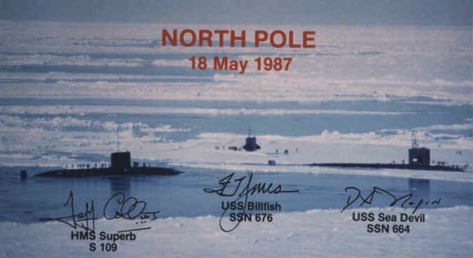
Fig.4 - HMS Superb, USS Billfish, and USS Sea Devil in a North Pole
rendezvous in 1987
(U.S. Navy Photo)
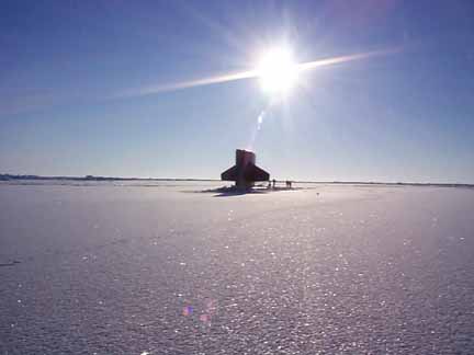
By contrast, a similar photo taken 12 years later of USS Hawkbill (with the ominous number SSN-666) at the North Pole during the spring of 1999 shows a vast expanse of unbroken new ice. (Hawkbill was nicknamed `the Devil Boat' due to its number, and was decommissioned in 2000 shortly after its last Arctic cruise, much to the relief of those familiar with the `Book of Revelation').

Fig.5 - USS Hawkbill at the North Pole, Spring 1999. (US Navy Photo) [19]
As early as 1959, the first US submarine to surface at the North Pole, the USS Skate, did so in late March, and surfaced at 10 other locations during the same cruise, each time finding leads of open water or very thin ice from which to do so. It did a similar cruise a year earlier in August 1958, again finding numerous open leads within which to surface. Here is a photo of the Skate during one of its surfacings in 1959. As can be seen in all three photos, the flat new ice is scarcely different between 1959 and 1999, while the 1987 photo shows the extent to which open water can occur.
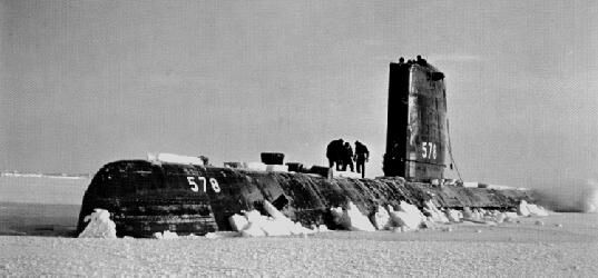
Fig.6 - USS Skate during an Arctic surfacing in 1959. (US Navy Photo) [18]
An aerial view of typical sea ice shows it to be a patchwork of ice slabs separated by areas of open water. In winter the ice will be more continuous as the ice free areas freeze over.
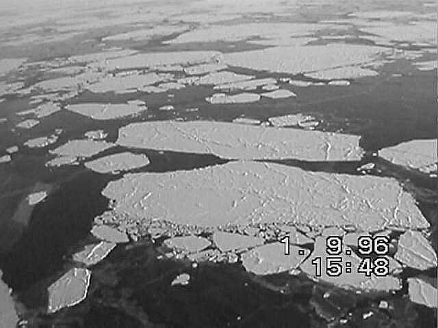
Fig.7 - Aerial view of typical polar sea ice.
In the rush to sensationalise the story, the New York Times and other media outlets failed to check whether the claims they were making were actually true.
For example, one crew member aboard the USS Skate which surfaced at the North Pole in 1959 and numerous other locations during Arctic cruises in 1958 and 1959 said: [5]
"the Skate found open water both in the summer and following winter. We surfaced near the North Pole in the winter through thin ice less than 2 feet thick. The ice moves from Alaska to Iceland and the wind and tides causes open water as the ice breaks up. The Ice at the polar ice cap is an average of 6-8 feet thick, but with the wind and tides the ice will crack and open into large polynyas (areas of open water), these areas will refreeze over with thin ice. We had sonar equipment that would find these open or thin areas to come up through, thus limiting any damage to the submarine. The ice would also close in and cover these areas crushing together making large ice ridges both above and below the water. We came up through a very large opening in 1958 that was 1/2 mile long and 200 yards wide. The wind came up and closed the opening within 2 hours. On both trips we were able to find open water. We were not able to surface through ice thicker than 3 feet."
Other scientists and experts on the Arctic environment quickly dismissed the McCarthy claims, pointing out that stretches of open water in summertime are very common in the Arctic [12]. Previous Arctic explorers even expressed frustration at being unable to proceed over the ice due precisely to unpredictable areas of open water obstructing their progress. The reason for the areas of open water is that the floating ice is subject to stresses from wind, currents and tides, causing cracking, ridging between slabs, and the creation of open leads of water between separating ice slabs. In winter, open leads quickly freeze over from the sub-zero air temperature, but in summer with the air temperature often above sea water freezing point (-2°C), such leads can remain open for extended periods.
In the end, the New York Times retracted the story. But we should not be too quick to blame them - it was IPCC scientists aboard the Yamal, particularly James McCarthy, who first started the scare story. The media simply took his word at face value assuming his scientific credentials would be sufficient authority to support the story.
Recent Data on Arctic Sea Ice
Although the `water at the North Pole' story was ultimately discredited, there is nevertheless evidence that Arctic sea ice has recently been thinning.
A study by Rothrock & Maykut [14] in 1999 compared upward-looking sonar data [20] from submarine cruises in the 1950s and 1960s with similar sonar data from cruises in the 1990s. The first phase data originated with these submarine cruises.
| USS Nautilus (widebeam) | August 1958 |
| USS Seadragon | August 1960 |
| USS Seadragon, USS Skate | July 1962 |
| USS Queenfish | August 1970 |
| HMS Sovereign (widebeam) | October 1976 |
The second phase, was conducted between 1993 and 1997 with US submarines USS Pargo (1993) (Fig.8), USS Pogy (1996), and USS Archerfish (1997), all of them making sweeps of the Arctic ice during the month of September.

Fig.8 - USS Pargo at the North Pole in 1993. (US Navy Photo) [17]
Since ice thickness varies according to the month of the year, the authors used a model to adjust data from the earlier submarine cruises to normalise all the data to September, the month used by the later submarines. This mismatch of dates between the various cruises introduces structural errors into the comparison in spite of the model adjustments. The data itself did not represent ice `thickness' as such, but `ice draft', or that portion of the ice below sea level. Since the proportion of ice which lies above and below the water line is well known, ice draft is a reasonable guide to ice thickness. However, it makes no allowance for snow depth lying on the ice.
Furthermore, not all the Arctic was
analysed in this way. For
security reasons relating to the Cold War, only the `Gore Box' was involved, a
roughly rectangular region of the central Arctic which the then Vice-President
Gore moved to have de-classified for purposes of sea ice data analysis. The
criteria for determining the boundaries of the `Gore Box' is not known but it
does introduce another layer of human selectivity into the picture.
After correcting and averaging the ice draft data for the Gore Box between the two periods, the authors concluded that -
"In summary, ice draft in the 1990s is over a meter thinner than two to four decades earlier. The mean draft has decreased from over 3 meters to under 2 meters".
A study by Wadhams and Davis [21] presented results from a British submarine cruise carried out in the Eurasian Basin in September 1996 in which it followed a track that was close to that of the HMS Sovereign cruise in September-October 1976. Comparing the sea-ice data from the two cruises, they found that mean ice draft from the Fram Strait (the wide waterway between Greenland and Spitzbergen) to the North Pole (81-90° N and 5° E-5° W) had declined by 43% between the two cruises. The Fram Strait is the primary inlet for warm Atlantic water.
One problem which these various researchers did not address was the effect of inter-annual variability on statistical trends. This means that if the ice draft data undergoes big swings from one year to the next, it may not be possible to establish clear trends for many decades due to the skewing effect of the more extreme years. The Wadhams study in particular was susceptible to this effect, since they compared two submarine cruises in only two widely separated years. Their conclusion that there had been a decline in sea ice draft between the two reference years could be as much due to inter-annual variability as it was to any genuine long-term thinning.
This problem of inter-annual variability was however addressed by McLaren et al [7], who analysed submarine data for the North Pole area over a 14 year period from 1977 to 1990. They found that ice draft varied up to 1 metre year to year, while the extent of open water was subject to a variation of 2.5%. This variability in thickness is close to the figure for overall ice thinning given by Rothrock & Maykut. McLaren et al also determined that the data errors associated with the averaging of the ice statistics was ±0.15 metres. To reduce errors even further, the McLaren team chose not to use the 1950s and 1960s submarine data, but instead chose only 6 submarine cruises `on the basis of data quality and because they were coincident in time and location'.
Sea ice researchers distinguish between `first-year ice' and `multi-year ice', first-year ice being newly formed, typically less than 1 metre thick, and covering the sea in extensive flat slabs. Multi-year ice is somewhat different in that it has been subject to a long process of grinding and breaking of slabs against each other over a period of time to form pressure ridges many metres tall, and matching `keels' many metres deep. Multi-year ice is distinguished by its deformed state whereas new ice is relatively flat. According to McLaren et al,
"The fractional coverage of multi-year ice also varies strongly on an inter-annual basis, for example from 27.1% in 1986 to 73.8% in 1987. These inter annual variations are sufficient to preclude definitive conclusions about recent changes in the Arctic maritime environment."
Before accepting claims of ice thinning at face value, it must
also be
understood that the sonar equipment used in the 1990s cruises were all `narrow
beam' sonars. But the USS Nautilus and HMS Sovereign from the
earlier period used `wide
beam' sonars. To compensate for this problem corrections were made to the data from these two submarines
by multiplying all their readings by a uniform adjustment of 0.84
With narrow beam sonar, the beam is readily able to pick out keels and troughs in the underside of the
ice, so that if the ice has an undulating subsurface varying between, say, 2 metres and 4 metres, the
sonar will `see' these undulations and the computer can make a reasonable average.
This is not true of `wide beam' sonar. With a wide beam, the sonar cannot discriminate between the peaks
and troughs in the ice, and instead returns an echo which only records the thickness at the peaks, so
that any statistical averaging will come up with 4 metres (i.e. the ice thickness at the peaks) but not recording the troughs or crevices in the way a narrow beam would do. In the example just given, a
correction of 0.75 would be needed, not 0.84. If the stated beamwidth correction is inadequate,
as seems likely, the Nautilus and Sovereign data will give the impression of observing thicker ice than in fact existed at the time.
This would then compare unfavourably with the ice more accurately measured by narrow beam
sonar in the 1990s.
Apart from these reservations about the boundaries of the Gore Box, inter-annual variability and the types of sonar used, it is nevertheless clear that some thinning of ice draft has taken place between the 1950s/60s and the 1990s. So, why has the Arctic ice thinned?
Fig.9 - Annual Mean Temperature at Jan Mayen [9]
In other words, these latest studies claiming significant thinning of ice between the 1960s and 1990s are comparing conditions during an anomalously cold period with the more historically normal conditions which exist today. Had the first phase data been collected a few decades earlier in the 1930s, it is likely there would be little significant difference in ice thickness between then and now.
As to why the 1960s and early 1970s should be so cold in the Arctic, it should be noted that it was on the Russian island of Novaya Zemlya deep in the Arctic that most of the powerful Soviet H-bomb tests were conducted in the atmosphere during the huge Soviet test series of 1961-1962, these tests being particularly large and dirty, the largest blast there being a mammoth 60 megatons on 30th October 1961 [11]. The cold plunge in Arctic temperatures occurred in the immediate wake of these tests, and it took about 12 years or so for temperatures to recover to their earlier levels. It is a strong possibility that the two events are connected.
Ice thickness is only part of the story. There is also the question of the areal extent of sea ice. This graph shows Arctic sea ice extent, based on satellite observation since 1973.
Fig.10 - Arctic sea ice extent 1973-1999 [10]
The total area of the Arctic Ocean is about 14 million sq. km. The above graph shows a significant shrinkage of ice extent during 1979 at the end of the Arctic cold period, amounting to almost 1 million sq. km., or 7% of the total. Since 1979, the ice area has largely stabilised, reaching a brief minimum around 1995, and increasing again since then. Put simply, the ice area today is scarcely different to what it was in 1979. This is consistent with observations that the Arctic atmosphere has not warmed since 1979. Had it warmed through the 1980s and 1990s, the ice area would have continued to shrink as increasing air temperature would have failed to re-freeze the ocean surface.
Interestingly, during the very same period, Antarctic sea ice increased in area by about 1.3% per decade [1], suggesting both polar regions are responding to regional factors rather than global ones.
The fact that we have observed recent ice thinning but not areal shrinkage of sea ice strongly suggests that the temperature of the atmosphere (and therefore the Arctic greenhouse effect) is not involved in the variations in sea ice thickness. A 1995 NASA study [3] also found a possible association between the El Niño Southern Oscillation and Arctic sea ice extent although this is not immediately obvious from either the sea ice data or the weather station records.
Why is the ice thinner?
This might at first seem an odd question since ice obviously melts if the temperature of the air or sea rises, thus making `Global Warming' routinely blamed for the thinning. But this would be a premature conclusion.
Try this experiment in any kitchen -
1) Take three identical ice cubes from the freezer compartment of the fridge
2) Place one cube in a large settled bucket of cold tap (faucet) water
3) Place a second cube in a kitchen sieve and let a slow trickle of cold water flow over it.
4) Place the third cube in a sieve and let a fast trickle of cold water flow over it.
In this experiment, the cold water from the mains water supply is at the same temperature throughout. But which ice cube melts away the fastest?
The ice cube in the bucket will take longest to melt. The cube under the slow trickle will melt considerably faster, while the cube under the faster flow will melt quickest of all. And yet, the water used to achieve these three different melting rates is at or near the same temperature.
The lesson this has for considering changes in Arctic sea ice thickness is that there is a deep water ocean several kilometres deep directly beneath the thin layer of surface ice. That ice can be thinned either by the atmosphere above the ice layer, or by the ocean beneath it. In the case of the atmosphere, the mid-summer temperature in the Arctic is barely at freezing point, insufficient to cause such large scale thinning. There has been little change in atmospheric temperatures in the Arctic over the last several decades.
Here is the September temperature record for Franz Josef Land, a Russian island deep in the Arctic only 600 miles from the North Pole, September being the month used by the 1990s submarine cruises and the month to which the earlier data was adjusted. The location of Franz Josef Land is shown in Fig.12.
Fig.11 - September mean temperature at Franz Josef Land (Russia) [9]
As fig.11 shows, there has been little change in September air temperatures since 1958, merely large year-to-year variations which are quite normal in the polar regions. Being the record for only one month of the year, the 1960s cold period is somewhat attenuated in this record. Since the Greenhouse Effect is a strictly atmospheric phenomenon, and since there has been no warming, that rules out greenhouse gases in the Arctic atmosphere as a factor in the ice thinning.
That leaves only the ocean beneath the ice. Being liquid, its temperature is above the freezing point of sea water, resulting in a continuous attack upon the underside of the ice. The faster the ocean flows beneath the ice, the faster is the melt rate, just as in the kitchen experiment.
The observation in the submarine studies of thinning ice cover, but with a largely constant area of ice, is consistent with changed flow rates of ocean water beneath the ice.
Where all the Water Comes From
Here is a map of ocean currents in the Arctic Ocean.
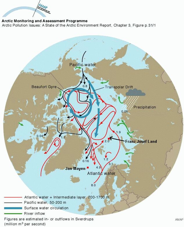
Fig.12 - Sources of Ocean Circulation in the Arctic Ocean [16]
As can be seen from the map, by far the greatest contribution of surface water comes from the North Atlantic, quoted as 8 `sverdrups'. Atlantic water flows in via the Gulf Stream which crosses the North Atlantic from the Americas, washes the coasts of northern Europe, and proceeds up to the Arctic, passing Jan Mayen Island and Franz Josef Land. As the water flows northward, it slowly cools. The faster the flow, the more warmth is retained by the water as it enters the Arctic. There is also a much smaller contribution from the North Pacific and adjacent continental river systems, but it is the Atlantic Water which is dominant.
Recall at this point the kitchen experiment with the ice cubes. If the surface Atlantic water flow increases, there will be greater propensity to melt sea ice from beneath. If the flow rate decreases, the summer ice melt rate is less and ice can become progressively thicker with each winter. `First year' ice tends to be thinner than `multi-year' ice and the thickness of the older ice is largely dependent on the flows of water beneath the ice and on the amount of ridging created through ocean movement and tides.
If the rate of flow is increased, not only will the melt rate increase (as per the kitchen experiment), but the water itself is likely to be slightly warmer as it enters the Arctic Ocean since it will have had less time in which to cool on its journey north. Thus an increased flow rate is also likely to be manifested by higher water temperature as it enters the Arctic. Results from several submarine cruises in the Arctic during the 1990s indicate that the influence of Atlantic water has become more widespread and intense in the Arctic, consistent with an increased flow rate of water through the Fram Strait and Barents Sea.
The North Atlantic Oscillation and Thermohaline Circulation
As to why there should be changes in the rate of flow of Atlantic water into the Arctic, it is necessary to consider what drives that flow.
The warm Atlantic water is basically subject to a `push-pull' action.
On the one hand, water is `pulled' into the Arctic by Thermohaline Circulation', the tendency of surface water to get colder as it migrates northward until it ends up colder than the deep water near the sea bed. When that point is reached, the surface water is more dense than the warmer deep water, resulting in the surface waters sinking. As it does so, the bottom water is displaced, forming a slow southward moving current along the sea floor. In this way, water entering the Arctic Ocean at the surface is balanced by deep water leaving the Arctic in the opposite direction.
Salinity of sea water is also a factor in the circulation. Surface water in the Arctic Ocean is typically about 10% less saline than the deeper water [15], which would tend to make the surface less dense than the deeps. This is caused by injections of fresh water from continental rivers and summer sea ice melt. Since fresh water is less dense than sea water, it tends to cling to the surface as it spreads outwards. It is the combined density effect of temperature and salinity between the surface and the deeps which determines the amount of thermohaline circulation which can occur.
Fig.13 - The start of Thermohaline Circulation
Thermohaline circulation is important for the global oceanic balance as the water leaving the Arctic weaves its way along the sea floor, right down the North Atlantic, into the South Atlantic, along the deeps of the Southern Ocean, finally upwelling in the Indian and Pacific Oceans. In fig.14, the warm surface water (red) sinks near the Arctic and returns via a deep cold water current (brown), resurfacing in the Indian and Pacific Oceans.
Fig.14 - Global Thermohaline Circulation
As surface water sinks in the frigid Arctic through thermohaline action, more water is `pulled in' to fill the void left by the sinking water.
Water is also `pushed' into the Arctic by the pressure of the Gulf Stream, and given added impetus by the prevailing south-westerly winds that sweep across the North Atlantic.
It is here that perhaps the biggest influence on the Arctic sea ice manifests itself - the North Atlantic Oscillation (or NAO for short). This oscillation in the balance of weather systems in the North Atlantic region has only recently been discovered and is analogous to the mighty Southern Oscillation in the Pacific Ocean (El Niño / La Niña). Just as the cause and timing of the Southern Oscillation is not yet known, the cause and timing of the NAO is also not fully understood.
The effects of the NAO however, are all too real. The key measure of the NAO is the `NAO Index', an index number to indicate when the phenomenon is weak or strong. The index is established by comparing atmospheric pressure at Akureyri in Iceland and at the Azores.
Where the pressure gradient is shallow, the index number is negative, and is manifested by weaker winds and storm systems in the North Atlantic. The result is less forward forcing of the Gulf Stream by the south-westerly winds. Where the pressure gradient is steep, the index number is positive, and is manifested by more frequent and more intense storms, stronger south-westerly winds, and thus more forward forcing of the Gulf Stream.
Herein lies the key to why sea ice thickness in the Arctic might be subject to variation unrelated to atmospheric temperature. Recalling the kitchen ice cube experiment, a stronger faster Gulf Stream driven by a positive NAO, enters the Arctic, retaining more of its warmth due to the faster trans-Atlantic passage of the Gulf Stream waters, and increases the rate of summer ice melt from beneath the ice. When the NAO is negative, the Gulf Stream is both weaker and slower, has cooled more by the time it does reach the Arctic - and the ice gets thicker in consequence.
Having suggested the mechanism, it merely remains to see what the NAO state has been during recent years. The NAO is reconstructed historically from atmospheric pressure records from Iceland and the Azores going right back to the early 19th century.
Fig.15 - The North Atlantic Oscillation winter index, 1825-2000 [8]
This chart shows clearly that the winter NAO was strongly positive from 1900 to around 1930, while its most significant negative period, the time when sea ice would be expected to increase in thickness, was during the 1960s, the very time when the first phase of submarine sonar measurements were being taken. Since then, the NAO has seen another strong period of positive index values, indicative of stronger south-westerlies in the North Atlantic, and therefore enhanced flow of warm waters into the Arctic Ocean resulting in a thinning of sea ice.
When the NAO finally reverts to negative values, as with any oscillatory system, the reverse will happen. Atlantic water will weaken, become cooler as it enters the Arctic, and melt less ice than the more aggressive positive mode of the NAO. In this way, ice thickness will vary according to a continuing cycle.
We can see the possible effect of the NAO in the ocean temperatures measured at the North Pole at various depths in fig.16 [15]
|
|
As we can see from fig.16, the ocean
surface temperature in the Arctic is largely unchanged from the 1950s
through to the 1990s. Also unchanged is the deep ocean temperature.
It is only around the 250 dbar depth (a `dbar' is roughly equivalent to a metre) that we find significant variation in ocean temperature. The `EWG Atlas' figures originate with Soviet surveys of the North Pole area from the 1950s to 1980s and only give average values for whole decades. The `SCICEX' data gives values for individual years in the 1990s and was collected by submarine cruises on scientific expeditions. The warmest SCICEX temperatures measured at this depth was in 1995, the coolest being in 1991. This variability in temperature originates with variations in the temperature of the warm Atlantic waters entering the Arctic and is unrelated to conditions in the Arctic itself. This variability can be achieved either through the Atlantic waters being warmer or cooler at their source, or through the rate of flow of those waters being changed by the NAO. |
If the Atlantic water flow rate is increased, assuming a constant rate of cooling, it will enter the Arctic Ocean at a warmer temperature than if the flow rate is slower.
Waters at this depth cannot be warmed directly by the sun or greenhouse effect as solar radiation penetrates only to 100 metres depth, while infra-red radiation from the greenhouse effect can only warm the immediate surface `skin' of the ocean.
Fig.17 - Radiation Absorption by the Oceans at Various Wavelengths
The Sverdrup radiation chart in fig.17 shows that solar radiation at visible wavelengths can penetrate the ocean readily, heating it directly at depths down to 100 metres. However, it also shows that as the radiation moves into the infra-red, the ability of the deeper ocean to absorb heat rapidly diminishes. Once we move into the far infra red where radiation from the greenhouse effect occurs, only the immediate surface `skin' of the ocean can absorb that radiation. For that energy to be absorbed down to deeper depths requires the assistance of surface turbulence to mix in the heat. If the ocean surface is not turbulent (as frequently happens in the tropics - the so-called `Doldrums'), energy collected from the greenhouse effect can only warm the top millimetre of the ocean, most of the heat being promptly lost again through evaporation.
It is for this reason that the variability in deep water temperature in the Arctic at around 250 metres depth can only result from variation in either the flow rate or the temperature of the Atlantic waters entering the Arctic, the flow rate being strongly influenced by the NAO. Atmospheric temperature changes in the Arctic itself can have no effect on deeper ocean temperature due to this inability of water to absorb infra red radiation beneath the ocean's surface skin or for surface turbulence to transmit the heat down to such depths.
Conclusion
As we can see from recent history, both the extent and thickness of Arctic sea ice is certainly subject to variation. But it would be a mistake to assume that a brief period during which the Arctic is in a thinning cycle is anything more than that - a cycle. We know from past history that it has been subject to earlier retreats as suggested by the opening quote from 1817.
Part of the problem lay in the fact that useful data on ice extent and thickness only dates from the 1950s, yet our temperature record from Jan Mayen Island at the edge of the Arctic shows that the Arctic was warmer during the 1930s than it was during the 1990s. Unfortunately there is no comprehensive ice data from the 1930s. Instead such data begins in the late 1950s, at a time when the Arctic was entering into the grip of a known cold spell. As that cold period ended, it is hardly surprising to find thinner ice during the latter warmer period.
There is also the strong correlation between the NAO and the state of Arctic ice, a strongly positive NAO in the last decade increasing the flow rate of warm Atlantic water into the Arctic, while it was predominantly negative during the cold period of the 1960s, resulting in a reduced flow rate of Atlantic water and thus a reduced propensity for ice melt.
The strong positive NAO of the last decade is not unprecedented. While some might wish to associate this with human-induced `climate change', it is clear from the NAO record that it was also strongly positive during the early decades of the 20th century and even earlier. In other words, the NAO is a real natural cycle, not a manifestation of `global warming'.
Variability in sea ice thickness has no implications for sea levels. Since ice sea displaces its own weight in sea water, thickening or thinning of sea ice has a zero effect on sea level.
The freezing Arctic air which descended on North America and Russia during the 2000 winter shows that the Arctic atmosphere has lost none of its frigid bite, thus ensuring further renewal of sea ice.
The limits on the thickness of Arctic ice are determined by how low the air temperature can get, and on how warm and fast-moving the subsurface water is. Air temperatures measured in the Arctic region show no recent warming, thus discounting the possibility that recent thinning of ice could be caused by atmospheric warming above the ice. Rather, the thinning of ice in the 1990s is clearly associated with a warming of the sub-surface ocean, as shown by the SCICEX data, caused in whole or in part by the strong NAO increasing the flow rate of Atlantic water into the Arctic Ocean.
There is nothing in the data to suggest anything but natural cycles at work.
References
1] Cavalieri, D. et al. Observed Hemispheric Asymmetry in Global Sea Ice Changes, Science, v.278, p.1104, 7 Nov 1997
2) Daly, J., The Surface Record: Global Mean Temperature and How it is Determined at Surface Level,
2000, at http://www.greeningearthsociety.org/Articles/2000/surface1.htm
3] Gloersen, P., Modulation of Hemispheric Sea-Ice Cover by ENSO Events, Nature, v.373, p.503, 9 Feb 1995
4] Hadley Centre, UK - http://www.meto.govt.uk/
5] Hester, James E., Personal email communication, December 2000
6] IPCC WG1, Third Assessment Report, Shanghai draft 21-01-2001 20:00
7] McLaren, A. et al., Variability in Sea-Ice Thickness over the North Pole from 1977 to 1990, Nature, v.358, p.224, 16 July 1992
8] NAO winter index chart - http://www.cru.uea.ac.uk:80/~timo/projpages/nao_update.htm
9] NASA GISS station temperature data from - http://www.giss.nasa.gov/data/update/gistemp/station_data/
10] National Assessment Synthesis Team (NAST), Climate Change Impacts on the United States: The Potential Consequences of Climate Variability and Change - Overview document, USGCRP, June 2000
11] Parish, Ken, The Big Bangs, http://www.john-daly.com/bigbangs.htm, 2000
12] Polar Science Center, Oregon State Univ. on Yamal event http://nsidc.org/NOAA/ULS_Drafts/
13] President of the Royal Society,
Minutes of Council, Volume 8. pp.149-153, Royal Society, London.
20th November,
1817.
14] Rothrock, D.,
Yanling Yu, & Maykut, G., (1999),
Thinning of the Arctic Sea-Ice Cover, Geophys. Res. Ltrs,
v.26, no.23, pp.3469-3472, Dec 1 1999
15] SCICEX chart - http://psc.apl.washington.edu/northpole/index.html
16] SEARCH Science Steering Committee,
Draft SEARCH Science Plan,
http://psc.apl.washington.edu/search/search_plan/Science_Plan_9.html, Polar Science
Center,
University of Washington, Seattle,
2000
17] USS Pargo photo, 1993,
from http://www.csp.navy.mil/asl/ScrapBook/Boats/Pargo.jpg
18] USS Skate 1959 surfacing - http://www.csp.navy.mil/asl/ScrapBook/Boats/Skate1959.jpg (photo)
http://www.csp.navy.mil/asl/Timeline.html#A1950 (legend on previous
page to the photo)
19] USS Hawkbill
photo, 1999, from - http://www.usshawkbill.com/scicex3.jpg
20] Upward-looking sonar http://nsidc.org/NOAA/ULS_Drafts/
21] Wadhams, Peter ; Davis, Norman R.,
Further evidence of ice thinning in the Arctic Ocean,
Geophys. Res.
Ltrs. v.27 , no.24 , p.3973 (2000GL011802), 2000
![]()
Return to `Still Waiting For Greenhouse' main page