The Svensmark factor represents the amplification of global temperature changes in comparison to the measured changes in direct solar radiative forcing. According to an observation-based hypothesis, the reason for this factor is that the intensity of cosmic rays which increase the cloud coverage, is strongly suppressed by solar activity (solar wind) [H. Svensmark and E. Friis-Christensen, J. Atmos. Solar-Terrestrial Phys. 59, 1225, (1997)]. A further contribution for irradiance amplification may be the fact that haze and clouds partly dissolve with increasing solar activity before the mixed ocean layer warms up and thus evaporation increases.

A best fit climate simulation using variable stretch factors for increasing solar and decreasing CO2 sensitivity was presented by Eric Posmentier, Willie Soon and Sallie Baliunas in [Global Warming – the continuing debate, ESEF (1998)]. In Fig.1+2 on p.164-165 (here combined) the authors show the observed global temperature change (11-year running mean), the best fit for GHG only, the best fit for solar only and the best fit for a combination of GHG with solar. Only 43% of the warming for the last century is to be allocated to GHG whereas 57% to solar.

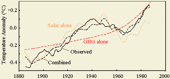
The authors found 1.8°C for CO2 doubling (alone), i.e. 0.8°C in proper combination with solar forcing – these figures denoting the equilibrium sensitivity. The transient figure for CO2 doubling alone was about 1.3°C. They have not applied corrections for aerosols – but as they considered the temperature increment to be even more than 0.7°C instead of 0.5°C, we can accept the result. Compare with Fig. 8.4c in [SAR, IPCC (1996)].

A similar paper was published by the same authors in [W. H. Soon, E. S. Posmentier and S. L. Baliunas, The Astrophysical Journal 472, 891 (1996)]. Another work coping with solar effects was the detailed paper "Implications for global warming of intercycle solar irradiance variations" [M. E. Schlesinger and N. Ramankutty, Nature 360, 330-333, (1992)]. The authors found 0.7°C for CO2 doubling in combination with solar variations by minimizing root-mean-square errors (see their Fig. 3). But by introducing a very high negative aerosol forcing, the solar effect reduced to 31% and the CO2 doubling soared up to 3.6°C.

Knud Lassen and Eigil Friis-Christensen reported in [Heuseler's Klima 2000 2, 17-20 (1998/9-10)] that P.M. Kelly and Tom Wigley published in "Solar cycle length, greenhouse forcing and global climate" [Nature 360, 328-330 (1992)] that simple energy balance models fit best to the observed data if it is assumed that there is only a solar impact (!). But the authors rejected this because the climate sensitivity to radiative forcing that was necessary to be assumed for this, would have yielded unrealistic (low) effects for the CO2 forcing.

Of course the Nature paper did not mention Svensmark or explicitly attribute solar impacts to the Svensmark effect. What the authors basically did was to multiply the solar climate sensitivity (in comparison to the direct forcing, equivalent to CO2 doubling) by a factor of x and use the changes in insolation. The CO2 sensitivity had to be lowered accordingly. The goal was just to find the best fit sensitivities, i.e. each DT for a DW/m². Here I cite some essentials of the paper:

• Greenhouse forcing considered alone:
> for history 1 (without aerosol forcing) the best fit occurs when delta T2x = 1.5°C... for history 2 (with aerosol forcing) the best fit occurs at... 3.7°C, as the global forcing is not great.

• Greenhouse and solar forcing combined:
> For history 1 and the KW solar record, the best fit occurs at delta T2x = 0.9°C and beta = -0.58. With history 2... 2.0°C and beta = -0.29.

• Solar forcing considered alone:
> No best fit occurs within the specified range of delta T2x.. The optimal pairing of beta and delta T2x is found at delta T2x = 25°C for the KW record and at delta T2x = 12°C for the FLC record... the visual correspondence between the simulated and observed temperature series is good... the overall credibility of the experiment with solar forcing alone must be considered low as it is illogical to neglect greenhouse forcing given the well-established case for its existence.

This statement is one of sensational logic. It reveals that IPCC (otherwise always keenly interpreting correlations) has committed a scandalous error in omitting a visually good correlation in favour of a visually bad one. To neglect greenhouse forcing, was not at all the question – this should be considered as unscientifical as neglecting solar forcing. The possibility that the climate sensitivity of CO2 might be indeed much smaller and then work out well together with an increased solar sensitivity, was purposely not considered. Good science would have postponed all climate simulations until these discrepancies were cleared.

The authors did not even mind that their aerosol cooling caused the CO2 sensitivity to increase up to 3.7°C. The doubling effect should be independent from aerosols – by correcting the temperature record for the cooling before the correlation analysis is done. Btw, MPIM Hamburg favoured 3.6°C equilibrium warming for 2*CO2 in 1998. Actually the aerosol effect is considerably less than it had been assumed [J. Hansen et al., Proc. NAS 95, 12753-58 (Oct 1998)].

Now allow me a rough layman's calculation. Say, the best solar-alone fit is 15°C and the best CO2-alone fit is 1.8°C. So the relative Svensmark factor should be about 8. If we take IPCC's 88% CO2 effect and 12% direct solar effect and divide the ratio by 8, we find that IPCC's relation between CO2 and solar should be rather 47% to 53%. In the Wigley paper the former equilibrium doubling effect of 2.5°C was already best-fit reduced to 1.5°C and then to 0.9°C with solar.

Apart from D. Hoyt and K. Schatten who empirically estimated 0.7°C/W/m² for the (transient?) solar effect in 1993, Dr. Landscheidt mentioned in http://www.john-daly.com/solar/solar.htm acc. to Prof. Claus Fröhlich, a mean value of 0.85°C/W/m² or for example 0.45°C (i.e. 0.16% of 288 K) for a change in solar irradiance of 0.22%. This provides us with the necessary figures for another calculation.

If we differentiate Stefan-Boltzmann for T, we get DT/T = 1/4 DS/S (assuming the Earth in radiative equilibrium). So to cause a temperature change of 0.16% the irradiance should change by 0.64% and not by 0.22% as observed. This means the Svensmark factor would be three in relation to radiative forcing. In 'solar physics news' [Nature 399, 416 (3 June 1999)]   Eugene Parker noted that a temperature increment of 1-2°C was observed in the northern temperate zone in association with a variation of solar brightness of about 0.5% and that DT/T is approximately equal to the relative change in brightness DB/B. So the Svensmark factor is about 4 – or even ~6 if we extrapolate from transient observation to the equilibrium effect. The question arises, why the Svensmark factor acc. to the Wigley and Kelly solar-alone simulation is eight.

There are data uncertainties, i.e. different records for solar activity and radiative forcing history and different grades of observation smoothing. Another problem is that damping effects for solar variations (caused by thermal inertia) feign a lower sensitivity (and may be correlation) than existing in reality (i.e. for equilibrium) whereas for CO2 the tendency is to use the known equilibrium sensitivity (including assumed water vapour feedback) and consider a smaller transient effect. The solar forcing is scaled to direct (transient) observation and thus becomes too small in relation to CO2 – so the ratio depends on the observed time interval and gradient of solar variation. It must be pointed out that best fit does not necessarily indicate best sensitivity, specially if single components of multifactorial effects and their time dependencies are considered.

Apart from these aspects the most obvious reason for a factor 8 is that the 'best guess' temperature effect of CO2 was about double of what it should be according to its radiative forcing. Analog to the solar Svensmark factor, we could call this the vapour factor of CO2. The 'best fit factor' x for solar forcing was chosen to obtain the temperature effect that would occur for CO2 doubling. So for properly equivalencing the solar impact within the climate simulations of the community, the relative Svensmark factor should be about 8.

This correction applied, yields a complete turnover of IPCC's projections which were so far based mostly only on CO2 equivalent. Reducing the CO2 doubling sensitivity of 2.5°C, using the best correlating solar fraction, would result in 0.8-0.9°C. Using this for calculating today's warming for a 50% equivalent increase of GHGs since beginning of the industrialization and taking a follow-up to 65% of the equilibrium temperature, we get 0.65*0.85*ln 1.5/ln 2 = 0.32°C. The fraction of 60% to be allocated to anthropogenic CO2, is 0.19°C. Because of aerosol cooling, the observed temperature increment is somewhat less (the solar contribution being subtracted).

The solar contribution can be calculated acc. to the Geophys. Res. Lett. paper by M. Lockwood and R. Stamper "Long-term drift of the coronal source magnetic flux and the total solar irradiance" http://www.wdc.rl.ac.uk/wdcc1/papers/grlcover.html. A very good correlation between magnetic field and solar brightness for the interval 1901-1995 indicates a rise in the average total solar irradiance of about 1.65 W/m² or 0.12%. Multiplied with the (transient) Svensmark factor 4 that is 0.48% and application of Stefan-Boltzmann yields a solar increment of 0.48%*288/4 = 0.35 K.

Concluding for a future CO2 doubling till 2100 (using my carbon cycle model, scenario IS92a and burning 1,500 GtC, i.e. even more than all fossil reserves except all available coal), we can expect about 570 ppm and a transient warming of 0.65*0.85 = 0.55°C for CO2 only, i.e. without aerosol effects and other GHGs. This is just 0.36°C more than today and by far within tolerable limits – apart from the benefit of a greener world by CO2 and N fertilization together with increased precipitation.

9 July 1999, Dipl.-Ing. Peter Dietze
Phone & Fax: +49/9133-5371
e-mail: 091335371@t-online.de
this paper: http://www.john-daly.com/fraction/fraction.htm

Subject: Re: New GW solar fraction paper
Date: Thu, 15 Jul 1999 11:37:37 -0800
From: "Warren B. White" <wbwhite@ucsd.edu>
To: 091335371@t-online.de

Dear Dr. Deitze,

We regard to the solar issue we here at SIO have been working with Judith Lean at NRL in demonstrating the solar irradiance changes on decadal and interdecadal timescales over the past 100 years are reflected in basin- and global-average temperature and heat storage in the upper ocean. Moreover, we found these basin and global average changes in heat storage in the upper ocean to be roughly consistent with Stefan-Boltzmann black-body radiation law; that is, to within about a factor of 2, when all the errors are taken into account. These results also suggest that about 1/3 of the global warming in the upper ocean over the past century is due to an increase of solar irradience of a few Watts per square meter. But this took place during the first half of the century. Global warming in the upper ocean over the last half of the century could not have been due to changing solar irradiance because it had no trend over this period.

Please refer to

White, W.B., D.R. Cayan and J. Lean, 1998. Global upper ocean heat storage response to radiative forcing from changing solar irradiance and increasing greenhouse gas/aerosol concentrations. J. Geophys. Res., 103, 21355-21366.

White, W.B., J. Lean, D.R. Cayan and M.D. Dettinger, 1997. A response of global upper ocean temperature to changing solar irradiance. J. Geophys. Res., 102, 3255-3266.

---------------------------------------------
Dr. Warren B. White
Scripps Institution of Oceanography
University of California,
San Diego 8605
La Jolla Shores Drive,
NH-346 La Jolla, CA 92037
Voice: (858)534-4826
Fax: (858)534-7452
Email: wbwhite@ucsd.edu

Subject: Re: New GW solar fraction paper
Date: Thu, 15 Jul 1999 23:46:05 +0200
From: "P. Dietze" <091335371@t-online.de>
To: wbwhite@ucsd.edu

Dear Dr. White,

thanks for your interesting comments to my solar fraction paper at Daly's. I think, the figure (by Eric Posmentier, Willie Soon and Sallie Baliunas) shows in detail the time intervals and relative magnitude of global warming contribution of solar and GHG (for individual best fit).

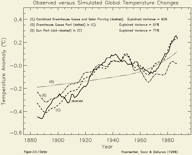
To show the combined fractions I append their Fig.3, presumably from the Astrophysical Journal 472, 891 (1996) [here combined with Fig.2]. As for each forcing a best fit factor (minimizing the sqared deviations all over the time period) has to be determined, one cannot simply say "first half century solar and second half CO2". You see that indeed from 1910 to 1940 the (positive) solar trend and from 1940 to 1970 the (negative) solar trend is dominant. Beyond 1970 both trends are positive, with CO2 being dominant. The warming percentages that I mentioned, were meant for the whole interval of industrialization, as given by the authors.

Btw, a similar figure you can see at "Climate Change Prediction" by Wallace Broecker [Science 283, 179 (8 Jan 1999)], where he combines CO2 with the (stronger) 200 yr solar cycle (amplitude ~0.25°C) and the (weaker) 88 yr Gleissberg cycle (amplitude ~0.15°C).

Sincerely, Peter Dietze

Subject: Re: New GW solar fraction paper
Date: Mon, 02 Aug 1999 08:35:47 -0800
From: "Gary D. Sharp" <gsharp@montereybay.com>
Organization: Center for Climate/Ocean Resources
Study To: 091335371@t-online.de

Hi,

I don't know what Doug Hoyt has published in the recent months, but I do know he has been busy. So contact him directly about his progress: <http://users.erols.com/dhoyt1/index.html>

He and others are using his solar index, including Leonid Klyashtorin, James Goodridge, and myself in a manuscript that we are preparing that shows the relations between LOD, Solar activity and Pacific Ocean SST patterns, rainfall, and global fisheries are all changing in synch.

Cheers, --

Gary D. Sharp
Center for Climate/Ocean Resources Study
PO Box 2223, Monterey, CA 93940 <http://www.monterey.edu/faculty/SharpGary/world>
831-449-9212
gsharp@montereybay.com

"The improver of natural knowledge absolutely refuses to acknowledge authority, as such. For him, scepticism is the highest of duties; blind faith the one unpardonable sin." Thomas H. Huxley

Subject: Re: New GW solar fraction paper
Date: Mon, 02 Aug 1999 10:41:09 -0700 (PDT)
From: ritson@SLAC.Stanford.EDU
To: 091335371@t-online.de

Dear Peter,

Thanks for your e-mail note. I used the four box Wigley UDEBM, Northern Land, N Ocean, S land, S ocean for similar fitting purposes, but fitted to the four boxes simultaneously. This is a substantially more constrained fit. Neither your solution or the Wigley Jones IPCC-95 solution survives this test. Basically the observed 1940 peak in the warming anomalies is largely derived from the Northern Ocean box. Your solution would spread it relatively equally over the four boxes, Wigley and Jones get their main contribution to the peaking structure from the Northern land masses (the result of their assumed strong Northern land aerosol effects strongly `interfering' with the GHG warming.) The preferred four box solution (though the errors are large) has a small aerosol component and a relatively small solar component. The residual fit errors mainly come from the Northern Ocean box, presumably a `natural' mutlti-decadal oceanic current fluctuation. The preferred climate sensitivity factor (again with wide errors) is about 1.5 deg C for 2xCO2.

I would naturally be interested in your reaction to the above,

Dave Ritson.
====================================================================
David Ritson, Emeritus Prof of Physics
Varian Physics Dept
Stanford University
Stanford, CA 94305-4060, USA

e-mail: ritson@slac.stanford.edu
Telephone number: 650/723-2685
FAX Number: 650/725/6544

Subject: Re: New GW solar fraction paper
Date: Tue, 03 Aug 1999 15:25:36 +0200
From: "P. Dietze" <091335371@t-online.de>
To: ritson@SLAC.Stanford.edu

Hello Dave,

thanks for your answer. Re your four box simultaneous fitting I cannot comment much as I don't know the details. May be you can send me a reference or URL. My daly/fraction.htm was based on 11 yr global running mean, the papers by Posmentier, Soon and Baliunas. In principle it is true that if you apply averaged sections (NH land/ocean, SH land/ocean), may be even individually corrected for aerosols (what these authors had not done), you get different least square solutions - even if you compute a constrained best global fit. But I suppose the great problem will be to have sectionalized solar forcing histories - while not being sure about the Svensmark effects (which may differ between land and sea). In any case, the more detailed splitting you use, the higher deviations you will find. Of course all non-fitting deviations are interpreted as internal variability - I suppose, Wigley even estimated the solar effect that he neglected, as internal fluctuation.

Best regards, Peter Dietze

Subject: Re: New GW solar fraction paper
Date: Tue, 03 Aug 1999 13:56:28 -0700 (PDT)
From: ritson@SLAC.Stanford.EDU
To: 091335371@t-online.de

Sorry this was simply an exploratory exercise and isn't written up. It was simply a generalized linear regression for GHG, Aerosols and solar. You did it for one averaged box, try it for four boxes solving for the three amplitudes (GHG, Aerosol and Solar.)

Yes, you can get quite spurious solutions if a problem is underconstrained. In your case the apparent fit to the solar is the results of an effect mainly present in the Northern oceans (surely not a solar signature.)

For the solar forcing to be dominant you would have to postulate or show that it qualitatively much stronger in the Northern oceans to agree with observation. (Main stream climatologists appear to write this off as a natural mid century fluctuation coupled with other effects.).

Wigley used the Hoyt and Schatten forcing history. (cf Proc Nat Acad Vol 94, pp 8314-8320, August 1997, Colloquium paper. It is on the WWW at the PNAS site. Wigley kindly supplied his actual code to me and I modified it for my own purposes.) Statistically, if you are using your data properly, you can never increase precision by coarse binning.

Dave Ritson