
EXECUTIVE SUMMARY
This paper, been prepared for the
SEPP 2nd TAR draft review workshop
on May 28-29 2000 and the meeting in the U.S. Capitol, Washington D.C.
on May 30, focuses on IPCC's three most essential modelling and core parameter
errors. The impacts on all modelling results would be so tremendous that
if the TAR would be corrected for these errors, there would hardly be any
more justification for it. So this paper addresses only few individual
TAR fallacies, but focuses on the nondisclosed flawed science it is based
on.
Solar impacts
Taking into account the impact of solar variability
on global warming, best fit studies have revealed that solar forcing is
amplified by at least a factor 4. By leaving out this 'Svensmark factor'
and using an exaggerated aerosol cooling, IPCC maintains a CO2
doubling sensitivity of 2.5 °C that is about a factor 3 too high.
Carbon cycle
Our global Carbon Cycle Model
reveals a half-life time of only 38 years for any CO2
excess. With present constant global CO2
emission until 2100, the temperature would only further increase by 0.15
°C. Scenario IS92a would end up with 571 ppm only. IPCC assumed that
far more fossil reserves would be burnt than being available. Using a flawed
eddy diffusion ocean model, the IPCC has grossly underestimated the future
oceanic CO2 uptake. Hardly coping
with biomass response, limited fossil reserves and using a factor 4 temperature
sensitivity, all this leads to an IPCC exaggeration factor of about 6 in
yr 2100. The usable fossil reserves of 1300 GtC burnt by 2090, merely cause
548 ppm – not even a
doubling. The WRE 650, 750 and 1000 ppm scenarios, projected until 2300,
are infeasible. Emission reduction is absolutely useless: the realistic
temperature effect of Kyoto till 2050 will be only 0.02 °C.
Radiative forcing
The additional IR absorption (being
evaluated here for CO2
doubling) is the energy source for global warming.
HITRAN transmission spectra – the fringes being by no means saturated yet
– can be used to compute this absorption, mostly occurring near ground.
A simple radiative energy equilibrium model of the troposphere yields an
IPCC-conforming radiative forcing which is here defined as the additional
energy re-radiated to ground. Coping with water vapor overlap on the low
frequency side of the 15 µm band, the clear sky CO2
forcing is considerably reduced to 1.9 W/m². With vapor feedback and
for cloudy sky the equilibrium ground warming will be about 0.4 to 0.6
°C only – a factor 4 to 6 less than IPCC's 'best guess' for CO2
doubling.
1. Solar impacts
The Svensmark factor
being estimated in this paper, represents the amplification of global temperature
changes in comparison to measured changes in direct solar radiative forcing.
According to an observation-based hypothesis, the reason for this factor
is that the intensity of cosmic rays which increase the cloud coverage,
is strongly suppressed by solar activity (solar wind) [H.
Svensmark and E. Friis-Christensen, J. Atmos. Solar-Terrestrial Phys.
59, 1225, (1997)].
A best fit climate simulation, minimizing root-mean-square
errors and using variable stretch factors for increasing solar and decreasing
CO2 sensitivity, was presented by Eric Posmentier,
Willie Soon and Sallie Baliunas [Global
Warming – the continuing debate, ESEF (1998)]. Fig. 1.1
shows the observed global temperature change (11-year running mean), the
best fit for GHG alone, the best fit for solar alone and the best fit for
a combination of GHG with solar. Though the temperature
correlation with GHG alone is very poor, GHGs are used as base for
IPCC's climate change modelling. The correlation is much
better with solar alone, but becomes excellent
with a proper combination of both. The fractions for the best combination,
yielding an explained variance of 92 %, are shown in Fig. 1.2.
Remarkable is that Tom Wigley and P.M. Kelly
published in "Solar cycle length, greenhouse
forcing and global climate" [Nature
360, 328-330 (1992)] that simple energy balance models
fit best to the observed data if it is assumed that
there is only a solar impact. But the authors rejected
this because the climate sensitivity to radiative forcing that was necessary
to be assumed for this, would have yielded unrealistic (low) effects for
the CO2 forcing "..given the well established
case for its existence". This reasoning is of sensational logic. It
reveals that IPCC (otherwise always keenly interpreting
correlations) has committed a scandalous error in omitting a visually
good correlation in favour of a visually bad one. To neglect
greenhouse forcing, was not at all the question – this should indeed be
considered as unscientifical as neglecting solar forcing effects.
So IPCC, so far only coping with a 12% solar fraction
[direct solar forcing, see TAR Technical
Summary Fig. 8] had to match for the missing strong part
of the solar signal in the observed temperatures by using an exaggerated
CO2 sensitivity in combination with "internal
variability" and a properly adapted far too high aerosol cooling.
Fig. 1.1: Best fit climate
simulations (E. Posmentier, W. Soon and S. Baliunas 1998)
Fig. 1.2 reveals that 57% of the warming for the
last century has to be allocated to solar whereas only 43% to GHGs (of
which about 60 %, i.e. 0.18 °C, is to CO2 – recently
found essential warming by soot and cooling by sea salt aerosols not yet
considered). Whereas the best fit sensitivity is 1.8 °C for
CO2 doubling (alone), it is 0.8 °C in proper combination
with solar forcing – these figures denoting the equilibrium
sensitivity which is by a factor three less than IPCC's.
The transient figure for CO2
doubling alone is about 1.3°C.
Fig. 1.2: Optimal fractions
for combination of forcings
Eric Posmentier et al. have not applied
corrections for aerosols – but as they considered the temperature increment
to be even more than 0.7°C instead of 0.5°C, we can accept the
result. Compare with Fig. 8.4c in [SAR,
IPCC (1996)] and Fig. 1.3 (see CCCMA
Canada) where the CO2 sensitivity and aerosol
impact is far too high, but the parameters being adjusted to compensate
for a far too small solar impact – the same as in the IPCC Tar (Fig. 1.4).
Details about the estimation of realistic sensitivity parameters see in
my paper Estimation
of the solar fraction and Svensmark factor.
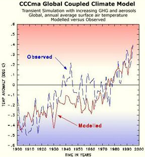
Fig. 1.3: CCCMA simulation
(G. Flato, G. Boer et al. 1997)
If we compare Fig. 1.3 and 1.4b with Fig. 1.2, it
is striking that for the interval between 1925 and 1970 when the solar
warming was high, IPCC models simulate a too low temperature and vice versa
around 1900. The "good match" beyond 1975 that IPCC emphasizes
upon, does by no means prove that the models are ok – the
match is a mere artifact, caused by a compensation between flawed
solar, CO2 and aerosol sensitivity parameters.
Fig. 1.4a reveals that IPCC erroneously assumes a
natural cooling after 1963 without GHGs (thus
the GHG warming being boosted). But in fact the solar
activity was increasing (see Fig. 1.2) which rather reduces GHG
warming.
Fig. 1.4: IPCC TAR-SPM Fig.
3 a) using primary solar and volcanic b) using GHGs and aerosols
How "useful" aerosols are to obtain any
required temperature curve – even when solar changes are left out, which
should result in gross mismatches – is shown in Fig. 1.5 [Meteorol.
Zeitschr. 7, 171-180 (Aug 1998)].
Fig. 1.5: Questionable statistic
aerosol climate simulation (C-D. Schoenwiese et al., 1998)
The same procedures are found with Tom Wigley
[Pew Center climate study 1999,
p. 15]. In Fig. 1.6 the far too high warming by CO2
in yr 2000 is cancelled out to 63 % (!) by aerosols
– the solar warming added, is flawed 21 % only. If IPCC believes in such
an essential aerosol cooling and being so concerned about the warming problem
from CO2, it logically follows that more SO2
would be the solution. So they could simply ask EPA to stop SO2
emission restrictions and permission trading in US. Kyoto could then be
cancelled – the problem would mostly solve without
economic impact, and billions of dollars could be saved.
Fig. 1.6: Pew Study: aerosols
compensate for 63 % of the exaggerated CO2
warming (T. Wigley, 1999)
2. Carbon
Cycle
One of the main reasons for
an assumed future CO2 disaster has been IPCC's assumption
that this greenhouse gas is accumulating
in the atmosphere – leading to the frequently
repeated 60% Toronto reduction demand.
But it is known that the oceans
contain about 50 times more carbon than the atmosphere, but may dynamically
take up only about 6 times more CO2 at equilibrium.
The photosynthesis of land biota may increase by up to 18 Gt C/yr for a
concentration doubling, i.e. three times today's
fossil emission. At present, the oceans are
still mostly on a pre-industrial level.
The IPCC's accumulation hypothesis
needs to be firmly contradicted. Supposed we pour water into a bucket that
has a hole. Nobody will state from observation that "about half accumulates
in the bucket". This fully depends on the hole, the water level and
how much water we are pouring.
The problem is easily solved
when the global carbon cycle is understood as a dynamic system in the manner
of control engineering. The atmosphere has a CO2 decay
function with a half-life time of about 38 years as will be shown in the
following. If the input function is doubling within the same time span
the system response would simply be a linear
concentration increase. The increase was misunderstood
by IPCC as a nearly irreversible accumulation
– one reason that led to hasty conclusions
for negotiating an unnecessary global reduction treaty.
A simple waterbox model can
be used to explain the atmospheric CO2
excess lifetime and to find a plausible value
(Fig. 2.1). The atmosphere is represented by a waterbox, filled up to a
level of 350 ppm (in 1988) with 743 Gt carbon (2724 Gt CO2
). This box is placed in a larger waterbox, representing the ocean.
Fig. 2.1: Waterbox model
for the excess CO2 lifetime
The atmosphere box has an outlet,
releasing about 2.7 GtC/yr into the ocean. The level decreases according
to an e-function if we postulate the transition flow is roughly proportional
to the water level difference or pressure. The lifetime
T can be defined as the time lapse until the
level goes down to 1/e (37%) against the equilibrium. The value for T can
be calculated dividing the amount of present excess by the present outflow,
yielding 55 years:
IPCC's 120 years had been erroneously derived from an arithmetic
mean of different sinks of the Bern model.
But the smallest
T (largest sink) is leading and a small additional sink flow (large T)
which would considerably increase the mean
value of T, is indeed decreasing
the resulting lifetime.
IPCC's eddy diffusion ocean
model (H. Oeschger, U. Siegenthaler, F. Joos, J. Sarmiento) is illogical
in assuming that a part of a CO2 impulse will be absorbed
straight away, another part fast at the beginning and then slowing considerably
(at the end e.g. to 360 years) and the rest, about 16%, to remain forever
in the air. CO2 impulses are continuously injected
into the atmosphere and nature should treat them all equally as it
cannot distinguish between 'old' CO2 to be absorbed
slowly and 'new' CO2 to be absorbed fast.
Thus the half-life time of 38 years has to be considered as an operational
overall value from observed sink flows at present conditions, assuming
the reservoirs are big enough and the system behaves in a roughly linear/proportional
manner within the operating regime.
Fig. 2.2: Electrical dynamic
CO2 model scheme (J. Goudriaan
1999 at daly/co2debat.htm)
explaining a 150 yr lifetime. Capacitors are Cs:
sinks, Ca: atmosphere and Cb:
buffer
A simplified linear carbon model scheme has been
presented by J. Goudriaan as an electrical circuit (Fig. 2.2). It
helps to explain essential flaws in IPCC's carbon model parameters, e.g.
a CO2 lifetime of 150 yr and
unduely coping with the fossil emissions part only. If we consider
Cs rather as infinite and add up the buffer Cb
and atmosphere Ca as C, we get the CO2
lifetime as T = R*C
= 50 ppm/Gt * yr *
(2.1+0.9) Gt/ppm = 150 yr. One reason
for this high value: the buffer is quite large (43% of the atmosphere).
So 30% of the (fossil only) emission, i.e. 1.5 GtC/yr, disappears
straight away into the buffer, erroneously considered as to be a
sink. So the remaining sink flow becomes 1.2 GtC/yr
only instead of the 3.6 what it really should be (see Fig. 2.1).
1.2 GtC/yr is indeed far too small for the ocean
and biomass together. This is why the modelled CO2
lifetime T is nearly trebled.
To develop a realistic dynamic
global Carbon Cycle Model, the waterbox model was extended, Fig. 2.3 showing
the transient state in 1988 containing no
missing sinks. Net photosynthesis of land
biota amounts to about 60 Gt C/yr, marine photosynthesis is roughly 20
Gt C/yr. The three upper boxes represent the land biota (650 Gt C), the
atmosphere (743 Gt C) and the mixed ocean layer (800 Gt C) which is closely
coupled with the atmosphere by precipitation and gas diffusion and exchanging
about 100 Gt C/yr with the atmosphere. In high latitudes the
icy cold salt water absorbs large amounts of CO2
. This makes the essential part of the net uptake (eddy diffusion as with
IPCC is indeed a minor part), the CO2 being taken
into the deep sea and mixing via the conveyor belt into all oceans. The
central link is the Antarctic Circumpolar Current. In warm upwelling regions,
especially where off-land trade winds are pulling up cold deep sea water,
we observe an outgassing of uptaken CO2
– the time delay being about 400 to 1000 years.
Fig. 2.3: Extended waterbox
model with proportional sink flows (numbers in GtC and GtC/yr for 1988)
Our sink flow approach does
not use IPCC's unrealistic eddy diffusion
model which leads to extremely small future uptake
but we use the basic diffusional mass transfer theory that can easily
be quantified by numerical-statistical treatment of well-known recent data
(compare the carbon
model of Jarl Ahlbeck). Given a high exchange
rate with big reservoirs, 95 % of the sink flows from anthropogenic perturbation
(so Ahlbeck) tend to be proportional
to the concentration increment against the
equilibrium state. For the system's differential
equation (box), being linearized around the
present operating regime, the concentration
increment in ppm can be calculated with a convolution integral
for the system being subjected to an arbitrary
total emission E(t) given in GtC/yr.

Here 0.354 = 1/(2.123*1.33)
is the conversion factor from GtC to ppm. For each 100 ppm the total buffer
excess C is 100/0.354 = 282 GtC, 212 GtC hereof being buffered in the atmosphere
and 70 GtC in surface water, soil moisture and fast-rotting biomass. We
will first consider a constant emission scenario
to demonstrate the model characteristics. For this case we get Dp
= 0.354 E*T*(1-e-t/T)
ppm.
Setting the total emission to be E=7 Gt/yr and T=55 yr, the concentration
will increase by 136 ppm for large t (Fig.
2.4).
The emission and concentration
start with the preindustrial equilibrium to perform a clean cold-start.
To match the actual concentration of 350 ppm in 1988 (with a sink flow
of 3.6 Gt), the constant emission of 7 GtC/yr is started here in 1948.
The concentration increases according to curve (a) as an e-function with
a T value of 55 years. The right hand vertical axis shows the model's proportional
sink flow reaching 7 Gt at a maximum concentration of no more than 416
ppm.
Fig. 2.4: Concentration
response and equilibrium temperature for
a) constant emission, b) after reduction to 50% in 1988 and c) after stopping
emission
At the start the airborne
fraction is 75%, which soon reduces to 36%
in 1988 and to 20% in 2020. The temperature scale shows an equilibrium
increment of only 0.32 K till yr 2100. After 1988 it is merely 0.15 °C
which shows that reduction claims are indeed unnecessary. Here the equilibrium
temperature increment is based on a (logarithmic) doubling sensitivity
of 0.6 K, i.e. a quarter
of IPCC's.
The dashed line at the upper
part of curve (a) is a hypothetical ocean equilibrium reaction for ideal
mixing after taking up nearly six times more CO2 than
the atmosphere, caused by the Revelle buffer factor (50/9 = 5.6). But in
fact this ocean response can be neglected as it will be mostly delayed
by several hundred years. The straight cumulation line shows how the IPCC
airborne fraction of about 50% would yield an increase up to 530 ppm –
an 80 % higher increment than in reality.
IPCC actually assumes about 500 ppm for this case.
Fig. 2.4 presents two further
scenarios. Curve (b) shows the response after reduction to 50 % emission
beyond 1988. As this amount equals the actual sink flows, concentration
and temperature remain quite constant. The increment from start is then
only 0.2 K and not 2 K (!) as has been assumed in early IPCC scenarios
even claiming a reduction by 60% until 2050, and as formerly documented
in the Greenpeace Report [J.
Legget (edt.), Oxford Univ. Press NY (1990)].
Curve (c) shows a hypothetical stop of emissions in 1988. The concentration
decays according to the e-fold lifetime of 55 years, the oceans and biomass
absorbing most of the CO2 excess within 120 years.
Discussing the effect of a
carbon and energy tax in Europe, an emission reduction of 4 to 5% has been
estimated – this means 0.7% worldwide. The
EU contribution for temperature reduction would be 0.7%
of 0.32 = 0.002 °C only.
But the projected taxation would be about
US$ 660 billion within 12 years. This seems
absurd as the effect is absolutely unnoticible.
According to a suggestion of
J. Goudriaan a numerical model test for total emissions during the
industrialization era till 1995 was carried out, using CDIAC data after
1970. In Fig. 2.5 the convolution integral
was sequentially solved by Excel in 5 yr interval steps and a good
replication of the Mauna Loa curve was obtained
– i.e. a concentration of 368 ppm for the
interval around yr 2000.
Fig. 2.5: Model test with
total emissions until 1995 and further acc. to IS92a
After 1995 emissions were applied
according to the business as usual scenario IS92a with piecewise
linear increments up to 20.3 GtC/yr in 2100. The concentration increases
rather linear
to only 571 ppm whereas IPCC's climbs to 700 ppm in yr 2100. The IPCC curve
(being parabolic)
has been approximated here by simply using a 47% airborne fraction.
Our model properly reproduces
the observed rather linear CO2 increment in spite
of a linear increase of emission – which (according to IPCC's flawed
accumulation hypothesis) should result in a quadratic
or exponential increment. Most interesting is the behaviour of the
airborne fraction f, here being defined as the ratio
of the atmospheric increment and the total emission (i.e.
not only fossil). At the beginning f is 1/1.33 = 75 % (see Fig. 2.1). For
1995 f is reduced to 35.3 % and in 2100 f becomes 19.8 %. IPCC models mostly
yield an airborne fraction of roughly 50 % that results in a far too high
future CO2 concentration – for
yr 2100 the increment is 50 % too high with IS92a.
IPCC mostly uses an exponential
increment of 1 %/yr for modelling i.e. doubling of forcing occurs
within 70 yr, though the TAR Technical summary (on p. 12) says that
the presently observed rate of CO2 increment is 0.4
%. For IS92a IPCC's CO2 increment is 0.62 %/yr.
How unrealistic a 1 %/yr CO2 increment is, can be
demonstrated as follows: With our model airborne fraction being 35 % in
1998, a total emission of 22 GtC/yr would be required
for a 1 % increment, whereas it was actually only about 8.3 GtC.
Debating the 1 %/yr assumption with David Schimel per email, he
emphasized that IPCC only carries out case studies,
mostly to test their models. The consequence is that IPCC
results cannot be interpreted as to be realistic future projections and
thus should not be (mis)used for political decisions.
The usable fossil fuels
(secured coal reserves, 4-fold gas and 3-fold oil being assumed because
of exploration and improved extraction) are estimated to be about 1300
GtC. With IS92a, this amount will be depleted until 2090. The CO2
concentration at that time only
reaches 548 ppm which is even less than doubling.
IPCC's CO2 increment to 700 ppm is by a factor 1.6
higher. Then, taking about four times the realistic temperature sensitivity,
IPCC has boosted the yr 2100
climate impact by about a factor of 6.
The 650, 750 and 1000 ppm WRE
stabilization scenarios shown in Fig. 26 and 27 of the 2nd
TAR draft, are definitely
infeasible. Until yr 2300 WRE 1000
would require about 3300 GtC, i.e. 2.5 times
more than available. IPCC obviously has only
created new scenarios but neither changed their carbon modelling nor coped
with limited fuel reserves. Their stabilization emission for
550 ppm remains 2 GtC/yr only (equal to the
sink flow). As in our model the total CO2 excess
for atmosphere and buffer is 784 GtC, the sink flow acc. to the 1/e lifetime
should be 784/55 = 14 (!) GtC/yr – IPCC's
is by a factor 7 smaller.
See as well the papers Little
Warming with new Global Carbon Cycle Model and discussion
and the German paper Der
Klima-Flop des IPCC.
3. Radiative
Forcing
The radiative forcing caused by a prescribed doubling
of the pre-industrial (or present or any)
CO2 concentration is the imbalance in the Earth's
radiation budget that is supposed to cause global warming. More CO2
means more absorption of the infrared (IR) re-radiation which the Earth
emits to space to compensate for the solar short wave irradiation. To restore
the radiative equilibrium between warming and cooling, the average 15 °C
ground which sends most of the thermal black body Planck emission directly
to space, has to warm up slightly until the withheld energy – i.e. in our
definition the increased back-radiation – is re-emitted.
The IPCC used the following definition, focusing
on tropopause level conditions:
"The radiative forcing
of the surface-troposphere system (due to a change, for example, in greenhouse
gas concentration) is the change in net (solar plus longwave irradiance)
in W/m² at the tropopause AFTER allowing the stratospheric temperatures
to re-adjust to radiative equilibrium, but with surface and tropospheric
temperature and state held fixed at the unperturbed values".
The often quoted additional absorption for CO2
doubling within the troposphere is not the forcing itself, as formerly
often (mis)understood by non-specialists, but it is the source of the (thermal)
re-emission to ground which is based on the atmospheric energy equilibrium.
This means, the re-emission at tropopause level plus the re-emission to
ground (which causes the warming) is equal to the additionally absorbed
energy.
Using HITRAN-1996 CO2 transmission
spectra from Jack Barrett, an Excel diagram (Fig. 3.1) was prepared
for a range of 300 cm^-1 and 560 intervals. It shows the transmission,
i.e. the intensity ratio T=I/Io
of an IR beam travelling from ground to the top of the troposphere, which
would be a layer of 6800 m for ground pressure. T depends strongly on the
wavenumber per cm (for example 15 µm means a wavenumber of 1/15*10^4=667/cm).
The data from HITRAN (high resolution transmission
molecular absorption database by L.S.
Rothman et al.) are extinctions E=-log(T)
(or line intensities, linestrengths) given per CO2
molecule for each individual peak wavenumber. The resolution is
extremely precise, about 0.0005 cm^-1. To cope with the optical density,
the molecular extinction is multiplied by the number of molecules (the
troposphere contains about 4.1 kg CO2/m²). HITRAN
integrates the linestrengths for each interval, coping with the peak shape,
pressure and temperature dependency – but the fact that nitrogen is not
neutral with respect to the CO2 IR absorption which
may be doubled, is omitted by HITRAN [H. Hug, CHEMKON
7, 6-14 (Jan 2000)].
The absorption is A=1-T.
The residual area in Fig. 3.1 (difference between the yellow 1*CO2
and green 2*CO2 spectra) is the
CO2 doubling absorption. Integrated to 16.8 cm^-1,
this is 6.4 W/m²
when multiplied with a medium Planck radiation of 0.38 W/m²/cm^-1
for 288 K in the range around 15 µm. The total absorption for 1*CO2
amounts to 74 W/m². Whether and how much N2
may effect the CO2 residuals, is not yet cleared.
This absorbed energy depends very little on the layer
thickness (optical density) and is thus not at all sensitive to the accuracy
of absorption within the troposphere (which was here simply powered up
according to the Lambert-Beer law, based on a 139 m equivalent probe, to
show the layer characteristics). Let us assume the residual absorption
for CO2 doubling to be 7.4
W/m² in total, coping with the missing part of the
yellow and green spectra at the left and right side of the diagram – here
considering as well the missing hot bands around 960 und 1064 cm^-1.
Fig. 3.1: HITRAN transmission
diagram based on data for 5% CO2
and 100 cm at ground pressure
The absorbed radiation is mostly thermalized and
dissipated (acc. to J. Barrett and H. Hug). In thermal equilibrium
this energy is re-radiated by atmospheric components as CO2
(double density yields double emission for the same temperature) and partly
by other GHGs – the latter only in case the temperature profile shifts,
contradicting the IPCC definition. In this case convective and latent heat
processes would become involved in additional vertical energy transport.
All these have to end up in thermal re-emission at tropopause level, directed
to both sides, space and ground. Whereas the
lower atmosphere warms, the upper atmosphere
is cooling (thus increasing
the lapse rate) – here doubled CO2 takes over
a part of the emission from the other GHGs.
As all re-emission has to be considered as being
bidirectional, we can assume in first approximation that half the total
re-emission goes to space and half goes to ground. So we yield the new
(by 15% reduced) IPCC TAR forcing of 3.7
W/m², as shown in Fig. 3.2. But the emission depends
on the 4th power of the absolute temperature. So if
we assume the bulk radiation temperature near ground (500m) as 285 K and
in the upper troposphere (5500m) as 255 K, the upper emission should be
only 64%. On the other hand we find very little water vapor in the upper
troposphere, whereas the vapor near ground considerably absorbs the CO2
emission. We have a mixture of up and down radiation, absorption and thermal
re-emission, normally being evaluated using the Schwarzschild radiative
transfer equation. Here we only consider the sum of re-radiation which
is known. As the correct ratio of the two emissions cannot easily be determined,
it seems reasonable to assume that the total emission is split about 1:1.
Important to mention that IPCC's forcing for
clear sky conditions is meant for well
mixed GHGs, i.e. without water vapor overlap [G.
Myhre, J. Highwood, P. Shine, F. Stordal in Geophs. Res. Letters 25,
2715-2718 (July 15, 1998)]. IPCC argues that at tropopause
level the water vapor density is negligible, which is true – but in reality
the forcing stems from absorption and back-radiation within the lower
troposphere near ground where we find the bulk of water vapor. As by
vapor overlap here practically the low frequency part (i.e. about 50%)
of the radiative forcing residual is cancelled (see below), we take 1.9
W/m² as radiative forcing (Fig. 3.2).
Fig. 3.2: Radiative fluxes
and forcing for CO2 doubling,
atmospheric thermal equilibrium model
Now the IPCC errors become
very obvious. Using the former forcing of 4.3 W/m² for tropopause
level, application of the differential form of the Stefan-Boltzmann law
dT/T=1/4*dS/S,
with S=240 W/m² and T=255 K, yielded a temperature increment of dT=1.14
K (which is now reduced to 0.98 K with 3.7 W/m²). The IPCC
assumed that this increment that doesn't exist as
the upper atmosphere is rather cooling, would be transmitted 1:1
down to the ground, based on a constant lapse rate. Because water vapor
is a strong greenhouse gas, the IPCC then used a factor of 2.2 as the effect
of water vapor feedback – neglecting that
on the other hand vapor should also reduce
the radiative CO2 forcing – and thus obtained a warming
of 2.5 °C for CO2
doubling, the 'best guess' – so called by
T. Wigley and S. Raper in a review
paper [Nature 357, 293-300 (1992)]).
D. Rind titled his article about the feedback approach "Just
add Water Vapor" [Science
281, 1152 (21 Aug 1998)].
But as observations did not support the exaggerated
warming, the IPCC assumed, the discrepancy was an effect of aerosol
cooling while other effects (e.g. amplification of solar forcing)
were considered to be insignificant. Their exaggerated aerosol cooling
and the gain in parameter variability was ideal to
maintain a far too high CO2 climate sensitivity,
thus compensating for missing solar forcing amplification and any other
model discrepancies, just as required.
Of course, the argument exists that the amount of
near ground moisture will increase with warming, and water vapor is a strong
greenhouse gas. This argument depends on IPCC's questionable assumptions
of total transfer of an unrealistic upper troposphere warming to the lower
atmosphere, and a strong water vapor feedback.
But here we have to consider a feedback
damping because the more IR is absorbed around 15 µm by water
vapor, the less remains for CO2 to be absorbed in
the same overlapping bands, and the water vapor absorbtion capability is
mostly saturated in this region of the IR spectrum, though not in other
parts. According to a mean ratio of 1.34 between
clear sky and cloudy sky forcing [Tab.1 and Tab.2 in G.
Myhre et al. (1998), see above] we can adapt our
forcing of 1.9 W/m² to 1.4
W/m² for cloudy sky condiditions. So at ground
level and 288 K with 390 W/m², the radiative
equilibrium warming of 0.35
K in Fig. 3.2 has to be
modified to 0.26 K,
any water vapor feedback not yet being included. We follow R. Lindzen
who claims a considerably smaller feedback and we assume a factor of about
1.6 (half of IPCC's). The ground warming would
increase to about 0.42 K,
a factor six less than IPCC's climate sensitivity.
The solar fraction analysis sensitivity (see above)
is by a factor three less than IPCC's 2.5
K. If we would assume a factor 2.2 for water vapor feedback, our doubling
sensitivity would become 0.57 K,
still 33% less than the solar fraction analysis figure. These values do
not require an assumption of enforced aerosol cooling because they provide
better agreement with observations than IPCC's 'best guess' sensitivity.
As most of the absorption for CO2
doubling occurs near ground – a doubling test for
139 m already yielded 6.5 W/m² (88% of
7.4 W/m²) – the water vapor overlap should mostly cancel
the left residual (and btw. some fraction of the right one as well).
H. Fischer has shown this in a graph of a position
paper of the German Meteorological Society (DMG), which advocates the
greenhouse effect. The "residuals" are the differences in transmission
between 1*CO2 and 2*CO2
(Fig. 3.3). We can estimate the cm^-1 area of the right residual (the left
was cancelled because the water vapor transmission is very small here)
and multiply with the associated Planck radiation per cm^-1. The radiative
clear sky forcing represented by this DMG residual is 1.7
W/m² only, of which 0.3 W/m² stems from the
hot band around 960 cm^-1. So our 1.9
W/m² forcing in Fig. 3.2 is likely. H. Fischer
used HITRAN data and apart from water vapor overlap he coped with other
greenhouse gases and with thermal CO2 emission depending
on atmosphere temperatures.
Fig. 3.3: German DMG residual
(H. Fischer, IMK Karlsruhe 1999)
IPCC authors so far refused to disclose details about
the modelling assumptions and computation of their core parameter, demanding
us to believe in their results – which is an unprecedented offence against
rules in public funded science, and the TAR again follows this line. A
graph about radiative forcing of the 1994 IPCC report is shown in Fig.
3.4. As the left residual is not cancelled, here obviously water vapor
overlap has hardly been considered, contrary to the statement in the note
on p.174 and the approach of H. Fischer. Each residual area in W/m²
from net irradiance at tropopause level roughly matches the one in Fig.
3.3 when logarithmically adapted to CO2 doubling,
though IPCC claims having even coped with cloud effects. R.D. Cess et
al. state in "Uncertainies in CO2 Radiative
Forcing in Atmospheric GCMs" [Science 262, 1252 (19
Nov 1993)] "The forcing is
substantially reduced through radiative overlap of the CO2
absorption bands by the absorption of water vapor" and "Clouds
also reduce the forcing".
Surprisingly the IPCC residuals (Fig. 3.4c) come
together at 15 µm, whereas in Fig. 3.3 they would be about 70 cm^-1
apart from each other. The IPCC residuals were calculated with radiative
transfer equations, using the standard narrow band code of P. Shine
1991 – both not been published by IPCC and obviously available within the
'community' only. Residuals show a broad gap inbetween when only absorption
is considered. Coping with thermal emission, they are shifted towards the
15 µm center – the more, if only a fractional layer (e.g.
upper troposphere) is evaluated. Their area (which is important)
only changes little. More details see at Estimation
of the Radiative Forcing for CO2 doubling and discussion.
Fig. 3.4: IPCC 1994 p.175
radiative forcing figure 4.1
In Fig. 3.4a IPCC did not correctly model the emission
characteristic to be seen in satellite measurements (Fig. 3.5)
which does not show a zero emission at the bottom of the funnel around
15 µm, but a thermal emission of about 120 mW/m²/cm^-1 (the
steradian-related value of 38 erg/(sec cm²) has to be multiplied by
p though one would
expect it to be 2p
for one direction). This left out emission, being about 4 W/m² for
the 1*CO2 base case, results
in a too high radiative forcing as it causes an increased part of the radiative
energy being withheld at tropopause level in case of CO2
doubling. The satellite clear sky measurements taken above Guam in 1970,
with added theoretical black body emission curves, clarly show the water
vapor impact below 575 cm^-1, a thermal tropopause CO2
emission peak from the bottom of the absorption funnel at 667 cm^-1, the
ozone absorption around 1050 cm^-1 and the methane and then water vapor
absorption beyond 1250 cm^-1.
Fig. 3.5: Satellite spectrum
(Kunde, 1974)
For a long time we had a controversial discussion
about discrepancies between satellite MSU measurements (about
1-5 km height, indicating hardly any warming trend), and ground
station readings, see as well http://www.john-daly.com/graytemp/surf-msu.htm#Dietze1.
Using IPCC's flexible aerosols, Ben Santer, Tom Wigley et al. tried
to model-experiment away and downplay this problem [Science
287, 1227-1232 (18 Feb 2000), see as well D.E. Parker on p.1216].
The warming effect from radiative CO2 forcing occurs
mostly near ground. So the GCMs which assume a parallel
shift of the troposphere temperature profile (as e.g. J.F.B.
Mitchell and Sir John Houghton formerly stated), instead of
coping with an increased lapse rate (see Fig.
3.2), erroneously assume a well and fastly mixed troposphere.
Even the 1st TAR draft Ch.6 p.6, line
52-54 still said that surface and troposphere are
closely coupled, the thermal structure being determined by
a nominal lapse rate, all thus behaving as
a single thermodynamical system. Because of the increasing lapse
rate satellites measure a mix of cooling and warming
and thus can principally not replicate the ground temperature trend.
Actually, if we apply proper physics, i.e. cooling
of the upper troposphere for increasing CO2,
and we use IPCC's constant lapse rate, the ground
should indeed be cooling (!) instead of warming. This demonstrates
one of the most absurd errors of IPCC.
H. Volz found an essential error source in
ground temperatures when calculating that the energy used in Germany, being
radiated off across the area of the country acc. to Stefan-Boltzmann, would
already cause an average temperature increment of 0.7 °C (!). This
increment remains rather constant as well as our energy demand and
does hardly increase with the CO2 concentration.
So this can neither be allocated to the CO2 increment
nor be subject to future CO2 projections. An energy
related ground bias may occur as the number of stations in developed and
energy intensive countries is quite large. It is not known to what degree
such effects have been corrected by IPCC.
4. Conclusions
The estimation of radiative forcing done here, shows
that IPCC's CO2 climate sensitivity has indeed to
be reduced considerably, just resulting in a rather harmless (if not beneficial)
warming till 2100. The corrections applied (as well as those for IPCC's
seriously flawed carbon cycle model), would completely turn over all simulation
results presented in the TAR.
The temperature trend of ground readings (especially
because of unreliable ocean surface measurements) should not be (mis)used
as a "proof" for the correctness of the highly erroneous CO2
sensitivity parameter on which the IPCC model results are based on. A considerable
part of the observed ground warming has to be allocated to amplification
of solar forcing (via cloud coverage), as well as to urban heating and
forest clearing (i.e. reduction of evaporation).
Within this century a reduction
of emissions is indeed not at all necessary, as in 2090 most of
the usable fossil fuel (estimated as 1300 GtC) will be depleted and the
CO2 concentration will not even be 550 ppm. When fossil
reserves become rare, technology can be expected turning to bulk power
production from fusion reactors and thorium breeders anyway. The latter
alone will be able to supply mankind with the presently used amount of
energy from oil and gas for 10.000 years.
A calculation of Tom Wigley (NCAR) [Geophs.
Res. Lett. 25, 2285-2288 (1998)] shows that for compliance
of developed nations with Kyoto, the temperature effect till 2050 will
be only 0.07 °C. As IPCC uses a far too high climate sensitivity, the
realistic effect should be about 0.02 °C only. Energy
and CO2 taxing within the EU will yield a contribution
for temperature reduction of 0.002
°C only. Contrary to the serious economic impacts,
the temperature effects of claimed emission reductions are absolutely negligible.
So the international bureaucratic activism to enforce Kyoto seems rather
useless and ridiculous. The planned emissions trading
requires the installation of a harmful eco-fascist
repression bureaucracy, CO2 counsils to allocate
emission grants and limits to individual industries and carbon taxes to
curb the folks. The permit to burn a ton of coal
beyond the limits may cost 150 US$, four to five times the price for importing
a ton of coal. Reporting and controlling facilities and drastic
punishments are required as well – being already planned in most details
(see the Greenbook
of the EU commission) – and the WTO will trade-sanction governments
that do not comply with the CO2 restrictions.
June 1st 2000, Dipl.-Ing.
Peter Dietze
Phone & Fax: +49/9133-5371
e-mail: p_dietze@t-online.de
This paper: http://www.john-daly.com/forcing/moderr.htm


Return to `Climate
Change Guest Papers' page
Return to `Still
Waiting For Greenhouse' main page